...
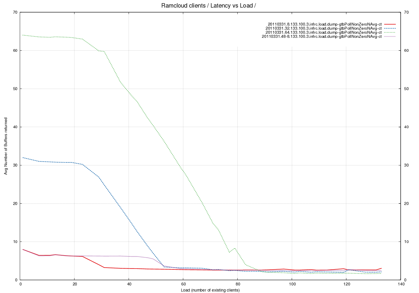
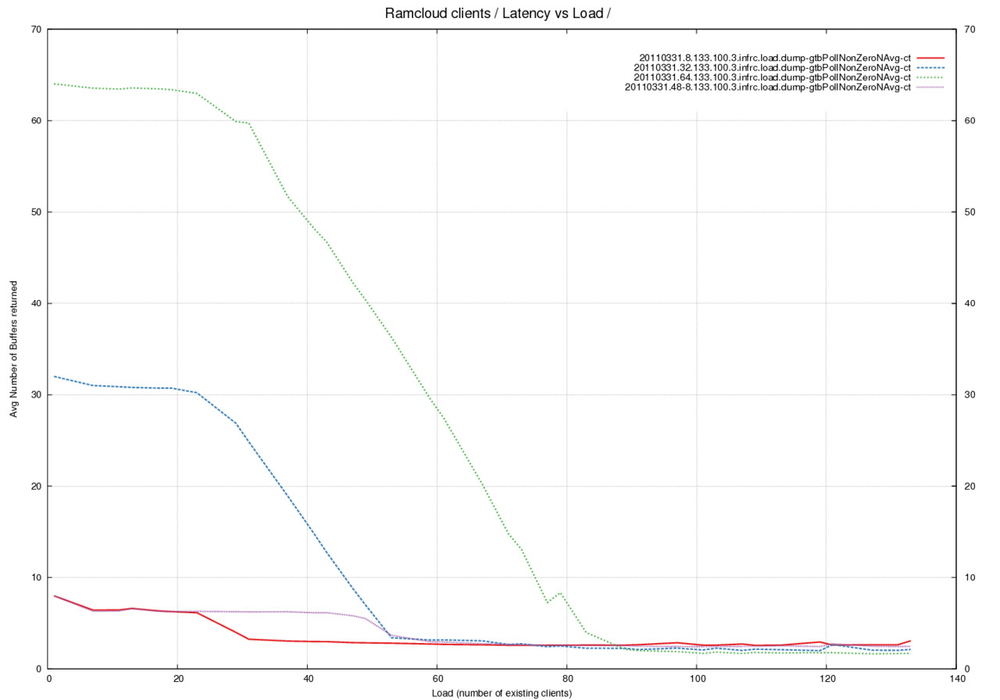
Latency Graph - Average number of buffers returned by pollCQ across different Buffer Pool sizes
Analysis
- This average does not include calls when no buffers were returned. This is an average when non-zero buffers were returned by pollCompletionQueue().
- The red, blue and green lines were measured with 24 RX buffers and
8, 32 and 64 TX buffers respectively. - The violet line was measured with 48 RX buffers and 8 TX buffers.
- An interesting trend that appears to be independent of number of
buffers in the pool. There is a drop in the average at the same load
irrespective of buffer-pool. - Why does doubling the number of receive buffers affect the number of
empty transmit buffers returned ? Compare Red against Violet. - Look at the average number of buffers returned under high load. It appears as if this number is around 3. We expect this number to be 1 buffer returned under load where empty buffers are returned as soon as they are available. The higher number indicates that maybe buffers are being returned in sets of 3. What is the reason for this behavior ?
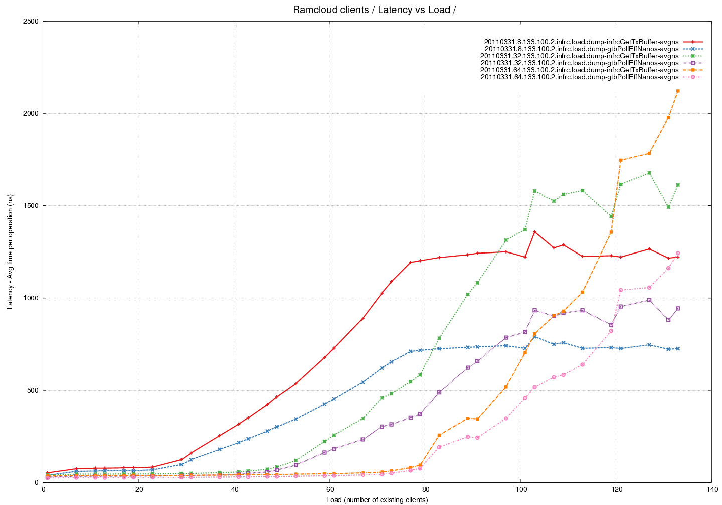
Latency Graph - Time spent in pollCompletionQueue per read (average) across different Transmit Buffer Pool sizes
Analysis
- Summary - pollCompletionQueue() (and hence getTransmitBuffer()) take
longer to run with increasing load. Note that pollCompletionQueue()
would be called multiple times until a succesful return - an empty
buffer from the pool. - Red/Blue lines represent 24 RX buffers and 8 TX buffers
- Green/Violet lines represent 24 RX buffers and 32 TX buffers
- Orange/Pink lines represent 24 RX buffers and 64 TX buffers
- This a plot of measurements of time taken by the different functions
during the experiments. - Total time spent in pollCQ was tracked and then divided by the
number of read calls to calculate the average. - This tracks the curve of time spent within the getTransmitBuffer
call well. The difference between the two needs to be explained.
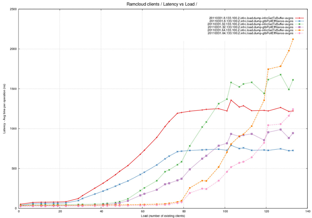
Latency Graph - Time spent in pollCQ per read (average) - fixed pool of buffers - comparing time taken by successful calls against calls that return 0
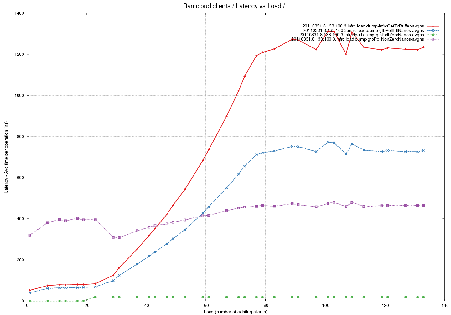
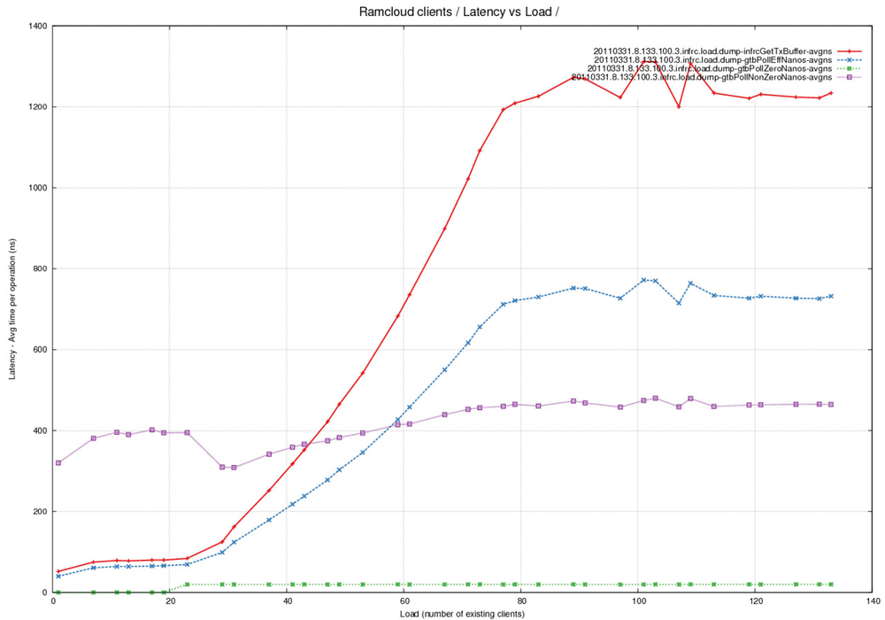
Analysis
- This is the same latency curve as above restricted to the case where
the size of the buffer pool for TX buffers is 8. - The Red line represents avg time taken by the getTransmitBuffer() call.
- The Blue line represents avg time taken across all the calls to
pollCompletionQueue() - The Green line represents the average time taken by calls to
pollCompletionQueue() calls that returned zero empty buffers. - The Violet line represents the average time taken by calls to
pollCompletionQueue() calls that returned non-zero empty buffers. - Note that time taken per successful call increased slightly with
load. Number of calls however increased with load resulting in overall
time taken by getTransmitBuffer() increasing.